These blog posts will build up into a complete description of a 2D marine processing sequence. They are based on our tutorial datasets, which in turn came from the New Zealand Government’s Ministry of Economic Development under the “Open File” System.
Following on from the previous post in this series - now that we have minimum phase shot records at a 4 ms
sample interval, we need to review the observer’s logs and do some quality
control checks on the data.
We’ve already covered a lot of the basics for a 2D marine line so we can focus now on the specifics of the seismic
line I’m working with:
- FFIDs are the same as
shotpoints in this case; from 100 to 975 with none missing
- There are 120 channels,
with channel 1 furthest from the boat. The group interval is 25 m, and the
near offset is 258 m. This makes the
far offset (119 x 25) + 258 = 3233 m.
When we sort the data to Common Depth Points (CDP), also
known as Common Mid Points (CMP), the “natural” CDP spacing is half the
receiver spacing; so in this case 12.5 m.
The number of traces in a CDP gather is referred to as the fold. This is sometimes expressed as a
coverage percentage: single-fold = 100% coverage, sixty-fold = 6000% coverage,
and so on.
Fold = (Receiver
Spacing x Number of Receivers) / (2 x shot spacing)
Fold = (25 x 120) /
(2 x 25) = 60
For more on seismic acquisition in practice, including fold
and CDP, visit this web page.
The first things to do are to look at the data – a few shots
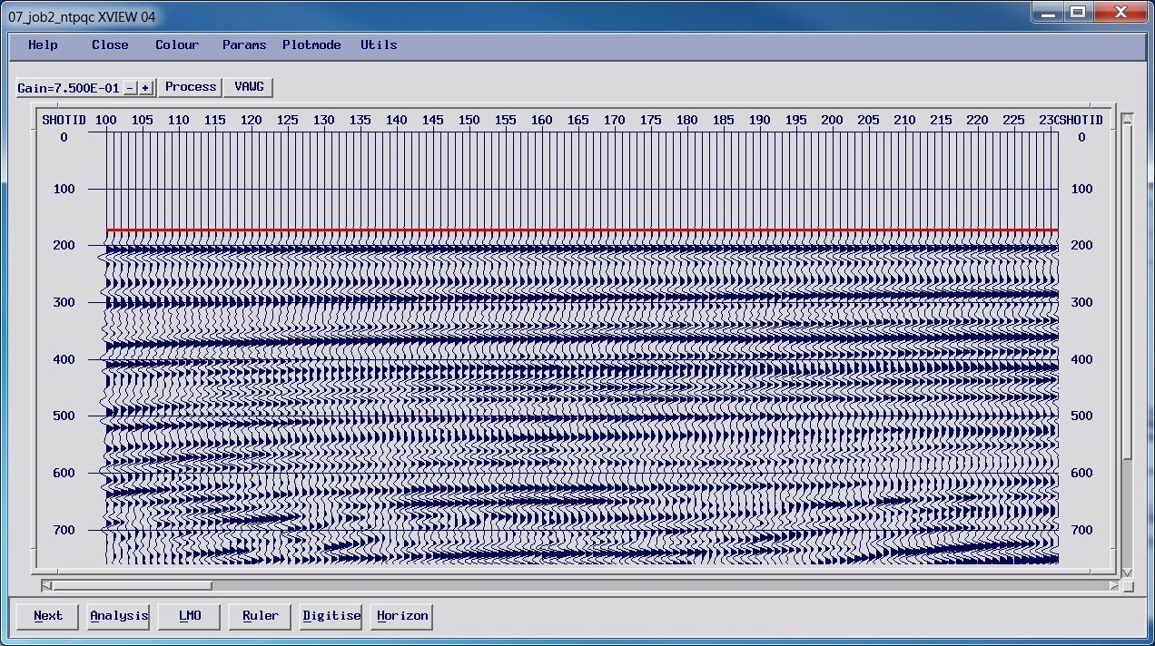
along the line and the near-trace-plot is a good start. Here’s what our shots look like:
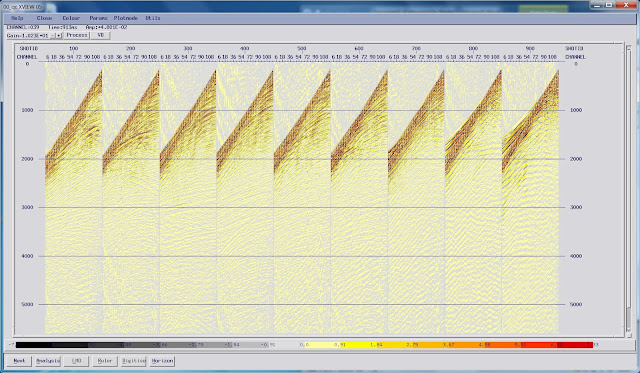 |
| Every 100th raw shot from the line with shotpoint number and channel labelled at the top |
There are only 120 traces per shot record, and no sign of
any traces that have a trace type not equal to one (trace type 1 = live), so we
don’t have to worry about any additional non-seismic auxiliary traces.
It is also a good idea to check the number of traces; in
this case I have 120 traces per shot, and (975-100) + 1 = 976 shots – so there
should be 117120 traces in total.
Looking at the data, there are actually quite a lot of
issues on these shots we are going to need to think about as we process the
line, partially because the geology is quite complex.
First of all the water depth is quite shallow, so much so that
you can’t easily tell apart the seafloor reflection, direct arrival and
refracted seafloor.
Looking at the direct arrivals and refractions, these get
quite a lot worse as we go from low shotpoint numbers to high ones; we also
seem to have more reverberations and lower frequencies on the high shotpoint
numbers. All of this suggests hard rock
with a high seismic velocity coming up towards the seafloor.
At time 4000 ms – 5000 ms, you can see some low frequency
rumbles; on shotpoint 200 there’s some energy that dips from the tail of the
cable down towards the head. This is referred to as “tailbuoy jerk” as it is
caused by the tailbuoy riding over waves and jerking the cable. There’s also
the “low frequency rumble” of swell noise.
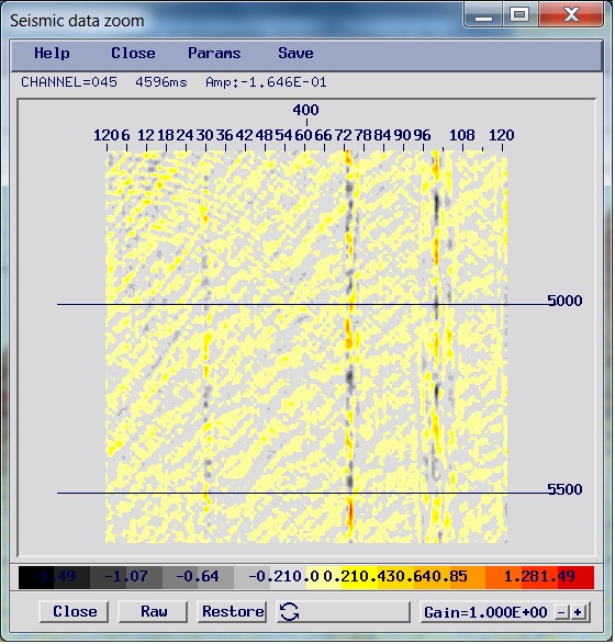 |
| Detail of SP 400: the low frequency, high energy "stripes" are swell noise |
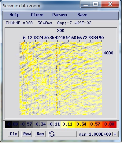 |
| Detail of SP 200: minor swell noise along with tailbuoy jerk, a low frequency dipping event (upper left to middle of the plot) |
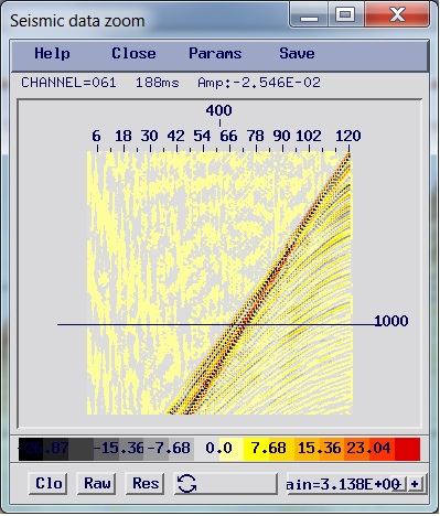 |
| Detail of SP 400: linear direct and refracted arrivals, as well as (hyperbolic) reflections |
 |
| Detail of SP 900: the faster (less steeply dipping) refracted arrivals, and loss of signal showing how the geology changes |
As part of the processing sequence we will have to manage
all of these – everything that is not a seismic reflection is effectively
noise.
The next thing we need to do is to sort out the geometry, so
that we can compare what we think the geometry should be to the actual data. In
most software the setting up of a 2D marine geometry is pretty simple – you
assume the streamer is being towed directly behind the boat (and so the offset
is a simple function of the channel number), and the CDP number is a function
of the shot number and the offset.
In our case the OFFSET = 258 + ((CHANNEL - 120) x 25), as
there are 120 channels that are 25 m apart and channel 120 is the near offset,
258 m from the source.
The midpoint between this near channel and the first shot is
129 m, or a little over 10 CDP spacings.
The midpoint between the far channel (at 3233 m offset) is
1661.5 m, or a little under 133 CDP spacings.
If we set the first CDP to be 100 (corresponding to the far
offset on the first shot), then the trace generated by the near channel will be
at CDP number 233. For the second shotpoint, we will have moved along by 25 m,
(or 2 CDPs) and so the far channel will correspond to CDP 102, and the near
channel will correspond to CDP 235, and so on.
There are a couple of things to note about this. If we take
two CDPs from the middle of the line (say CDP 400 and 401), then they look like
this:
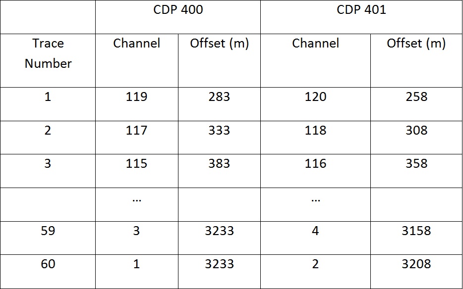
- Odd and even CDP numbers have different offset values, but the same number of traces
- The spacing between traces in the CDP gather is 50m, i.e. every second receiver
- The even CDPs don’t have the “near offset” trace in them
- The odd CDPs don’t have the “far offset” trace in them
This pattern becomes important later on in the processing
sequence, especially for processes that work on common offset planes.
Having assigned the offsets, there are three things we can
look at as a check:
- shots
- the near trace plot
- a “brute” stack
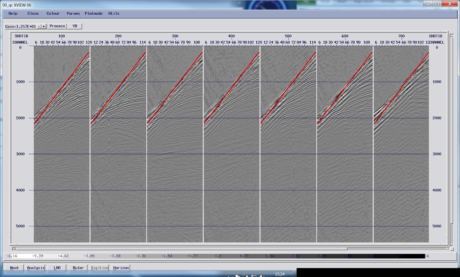 |
| Shot records displayed with the direct arrival time calculated from the offset (displayed as a red line). In this case the speed of sound in seawater (1500 m/s) was used to convert the offset in metres to a two-way-time value |
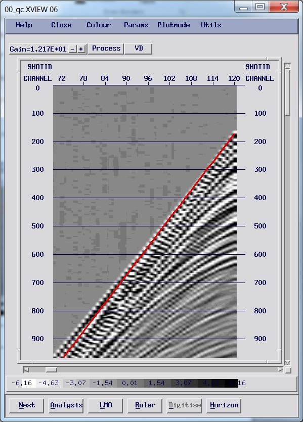 |
| Offset (red line) overlaid on shot record; it matches the first break, meaning it is correct |
On both the shot record and near trace plot displays, we can
calculate the time of the theoretical direct arrival based on the offset and
the speed of sound in seawater, which is usually in the range
1480-1500 m/s. By plotting this as a line
on top of the seismic, we can verify the offsets and the timing of the shots.
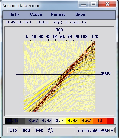
 |
| Part of the near-trace (channel 120) plot with the predicted time of the direct arrival (as calculated from the offset - displayed in red); this aligns well with the first arrival of the data, confirming the near offset and the absence of any gun delay |
To create a “brute” stack you will need a basic velocity
model; this should be a single simple function. The velocity model is often drawn
from some regional geological information – you may also have the capability to
make some rough velocity measurements with a “hyperbolic” ruler on the shot
records, for example. You could also output semblance spectra from the shots
and pick a velocity model from that, to be used to create a brute stack.
The basic approach is to gather the data by CDP number,
flatten the hyperbolic reflection events using the normal moveout (NMO) correction, and then stack (sum) the data to improve the signal to noise ratio.
The sequence is:
- Read in the minimum phase data at 4ms sample interval
- Apply the geometry we have defined
- Sort the data to CDP
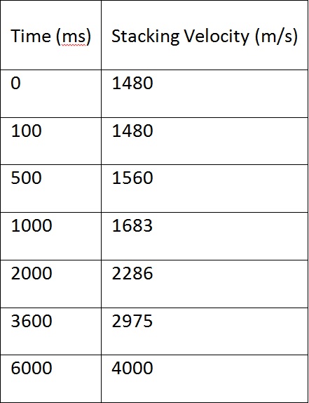
- NMO correct with a simple function
- Stack the data
When you apply the NMO, you can use an “automatic” stretch
mute at this stage. These are used to avoid low frequency artefacts on the data
when the NMO correction is large in the shallow portion of the section. As a side effect, they will also tend to
remove refracted data.
In this case I’ve used a velocity
function that has only a few points:
The “brute stack” gives an initial look at the structure of
the line; it is a good idea to plot the “fold” of coverage (the number of
traces in each CDP) on top of the stack as a check.
Now we have the geometry resolved and checked, we can start
to look at the data in more detail, and start to test some different processing
sequences to make improvements.
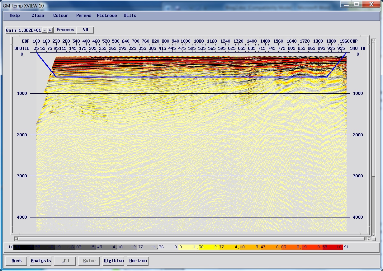 |
| The brute stack of the line, with the fold pattern overlaid (multiplied by 10); the data is un-scaled but you can still see the basic geological structure. The CDP numbers and shotpoint positions are both labelled. |

By: Guy Maslen